
Perceptra
Perceptra: A New Approach to Pattern Classification Using a Growing Network of Binary Neurons (Binons)
Abstract
Perceptra is a simple pattern classification algorithm that uses a compositional hierarchy of binary neurons called binons. Each binon represents a class or category. General categories are lower in the hierarchy and more specific combinations of categories are higher in the hierarchy. In this respect, binons are similar to perceptual schemata in schema theory or category prototypes / clusters in implicit category learning. When grounded, they are a possible implementation of Barsalou’s perceptual symbols (Barsalou 1999). For pattern classification the lowest level binons represent features extracted from stimuli. These features are the invariant shape and contrast patterns formed from the ratios between the widths and intensities of the perceived objects. These ratios are calculated by subtracting the logarithms of their values as described in the Weber-Fechner Law. Perceptra starts out with no binons and adds new binons to its network based on the coincidence and novelty of the features and their combinations. Its simplicity allows it to scale well over multiple levels of abstraction. It is sense independent and multimodal. It can recognize patterns of objects independent of their position, width and intensity. It has achieved over an 80% recognition rate on handwritten digits mapped onto a one-dimensional array of sensors.
Introduction
Machine learning is a branch of artificial intelligence in which computer programs learn from experience to perform tasks. Pattern recognition is a subset of machine learning in which the task is to learn the properties of objects and use this knowledge to predict the properties of unfamiliar objects. Pattern recognition performed by animals is called perception. There are three approaches to pattern recognition: regression analysis, pattern classification, and sequence labeling. Regression analysis is used to derive numeric results from source data. Pattern classification is used to predict the classes of objects. Visual pattern classification is called object categorization (Dickinson, 2009). In cognitive science, pattern classification is synonymous with implicit category learning. Sequence labeling is used to recognize patterns over time as in speech recognition.
The goal of this paper is to describe a new approach to pattern classification called Perceptra. Its development is based on the requirement for a simple and deterministic algorithm. It uses an incremental / growing, deep learning, and compositional hierarchy of binary neurons to represent categories. It makes no use of stochastic inference or tuned weights.
Approaches
There are many approaches to pattern classification that incorporate the concepts of growing networks, deep learning hierarchies or compositional structures.
Constructive neural networks are growing, feed-forward artificial neural networks (ANNs) that add layers, nodes and weights as learning takes place (Sarma & Chandra, 2010). Other growing neural networks have recently been reviewed. (Chaudhary, Ahlawat & Bhatia, 2011). [Another neural network that grows by adding nodes is the Cascade-Correlation Learning Architecture described by Fahlman and Lebiere (1990). This was not mentioned in the original paper] In cognitive modeling, category learning has a long history. A recent and most successful network model of human category learning is SUSTAIN. (Love, Medin, & Gureckis 2004). It begins with a single cluster / category and grows by adding more in response to surprising events.
Deep belief networks are hierarchical multi-layered ANNs. One approach uses successive layers of binary latent variables and a restricted Boltzmann machine to model each new level (Bengio, 2009). Convolutional networks are another approach. They use the techniques of local receptive fields, shared weights, and sub-sampling to ensure that the first few layers of a hierarchical network extract and combine local features in a distortion-invariant way. This overcomes the need to handcraft the feature extraction part of an object categorization algorithm (Fukushima, 1988; LeCun, 2012). Convolutional networks are fixed in size before training. Among all the many pattern classification algorithms, convolutional networks are proving to be the most successful (LeCun, Bottou, Bengio, & Haffner, 1998).
Hierarchical approaches have also been successfully used in probability based associative memory (Starzyk, He, & Li, 2007), Support Vector Machines (Cesa-Bianchi, Gentile & Zaniboni, 2006) and Self-Organizing Maps (Jlassi, Arous, & Ellouze, 2010; Kohonen, 1998).
There are some approaches that explicitly focus on the compositional structure and the coincidence of features to build hierarchical networks (Fidler, Boben, & Leonardis, 2009; Hummel & Biederman 1992). Bienenstock and Geman wrote this about composition: “Organization by composition is, in fact, so ubiquitous as to suggest that it is fundamental to cognition.” (Bienenstock & Geman 1995).
Most of the approaches mentioned above are not simple. They all involve some form of statistical or complicated mathematical functions to perform back-propagation / gradient descent or recurrent feedback. Learning is accomplished through the updating and tuning of weights. Although many take advantage of deep learning by using hierarchical, multi-layered networks, most use a fixed structure.
Perceptra is a simple pattern classification process that learns by continuously growing a compositional hierarchy of binary neurons (binons). The lowest level binons in the network represent the different types of shape and contrast features obtained from the stimuli. The mathematical functions of subtraction and logarithms are used at this level to calculate the relative values of object widths and intensities. At all levels, learning takes place by growing the binon network structure.
The next section describes binons and their network. Then the section on grounding the network describes how the types of features are represented in binons from the patterns of sensory data. A section detailing the classification process follows. The results section documents the success in using Perceptra for recognizing handwritten digits. The paper finishes with a discussion and conclusions.
[Key features of this approach are at the bottom of this page.]
A binon is a node that represents a class or category (also known as a kind or type of object). It has two ordered links, each to a lower level source binon, as in Figure 1.
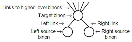
Figure 1: Source and target binon network structure
Binons form a binary hierarchy when viewed from top to bottom. All the connections are “has-a” / “consists of” links. Therefore, a binon network is a very restricted form of semantic network (Barnden, 1995). As a compositional hierarchy it is a simple form of conjunctive coding (Hummel, Holyoak, Green, et al, 2004). Each binon represents a specialized category made up of two more general categories. As an example, one source binon could represent heavy objects and a second represent wide objects. The target binon that is composed of these two would then represent the more specific category of heavy wide objects. Two source binons are said to be associated when they are linked to the same target binon. Note this is a compositional hierarchy, not a taxonomical, generalization, inheritance or an “is-a” hierarchy.
A source binon may be connected to zero or more target binons at a higher level. In this direction, the connections are “is part of” links. This forms what Fuster calls a heterarchy from bottom to top (Fuster, 2003). The more general categories (source binons) are shared and can be reused in the creation of any number of higher-level more specific categories (target binons). For example, the generic source binon for jointed legs could be part of more specific target binons representing birds, insects and walking robots.
Binary links between nodes in a hierarchy allow for the formation of many possible configurations. Figure 2 shows three ways in which three level 1 source binons could be combined to form a single representative node at level 3.
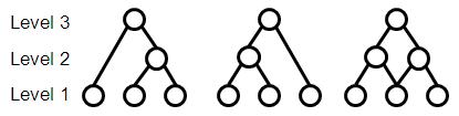
Figure 2: Hierarchies for representing three level 1 binons
The right-most structure in Figure 2 is preferred because it represents both pairs at level 2 and the triplet at level 3 while restricting links to adjacent levels. The result is a uniform compositional lattice that is simpler to build, as in Figure 3. As an example, red heavy wide objects at level 3 are represented as the combination of red heavy objects and heavy wide objects at level 2. This compositional structure is the only one used when combining binons in a network.
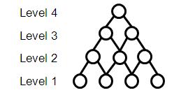
Figure 3: Compositional lattice
The binon network is the long-term memory for representing and recognizing categories of objects. But the lowest level binons must be grounded on sensory data extracted from the stimuli provided. The initial version of Perceptra works with a one-dimensional array of sensory data. Each stimulus is a list of intensity values as measured by this array of sensors, as in Figure 4.
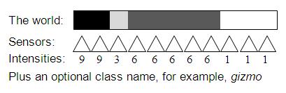
Figure 4: An 11 sensor stimulus & class name example
In this example, the values are graduated. They have a finite resolution on an interval scale. Although the world is presented visually in the example, the sensors could just as easily be auditory, haptic or from some other sense. If this were the sense of hearing each sensor would be tuned to a different frequency and the intensity would be the volume. For supervised training purposes a class name must accompany each stimulus.
In Figure 4, there are four parts that make up the gizmo. From left to right these parts have intensities of 9, 3, 6 and 1 and widths of 2, 1, 5 and 3. To represent the left most part a binon could be formed from two source binons, one for the intensity of 9 and the other for a width of 2. But the second part (intensity 3 and width 1) could belong to the same category as the first, just further away and not as bright. Because a part’s intensity and width can change, these properties are not useful features for identifying its category. The only invariant properties at this lowest level for categorization purposes are the relative intensities and relative widths between adjacent parts. The relative intensity between two parts provides a contrast ratio and the relative width of two parts provides a shape ratio. These ratios are the smallest possible and most generic patterns that are useful for categorizing an object.
Since a stimulus results in two independent property types (intensity and width), two separate binon hierarchies are formed, one for contrast patterns and the other for shape patterns. These are illustrated in Figure 5 and 6.
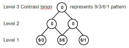
Figure 5: Contrast patterns - ratios of adjacent intensities
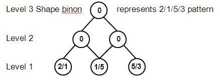
Figure 6: Shape patterns - ratios of adjacent widths
The binons in these hierarchies are called property binons because they are based on a single property type. The ratios are kept in level 1 binons. Since the structural nature of the ordered links to the source binons represents higher level patterns, values in higher level binons are irrelevant and are set to zero. Note there are no links between level 1 binons and the sensors. The level 1 ratio values are derived from the sensor information, allowing level 1 binons to be position independent. Perceptra starts with no binons. Level 1 binons are created whenever new ratios are found.
Most animals cannot and have no need to tell the difference between similar ratios such as 100/120 and 100/121. Therefore to simplify the binon network, Weber’s Law (Weber, 1850) is applied. It states that the just noticeable difference (JND) between two stimuli is proportional to the magnitude of the stimuli. This applies when one tries to distinguish between two graduated values. For example one would find it hard to tell the difference in width between two objects of 100 and 101 centimeters. However when the difference in width reaches 20 centimeters, for example, it becomes noticeable.
Fechner (Fechner, 1966) stated the same principle in mathematical terms. Fechner’s law states that human subjective sensation is proportional to the logarithm of the stimulus intensity (Portugal & Svaiter, 2011). This principle can be applied very economically to save having to represent ratios that are not noticeable or too similar to notice.
First, a ratio can be represented as a single value by using the logarithmic formula
log(a/b) = log(a) – log(b)
Second, if the result is converted into an integer then any two ratios that produce the same result have no noticeable difference. Mathematically, to obtain an x% JND a log base of 1 + x/100 is used. Thus, a log base of 1.2 will provide for a 20% JND. As an example, using a 20% JND all the ratios from 100/101 up to 100/119 produce a zero result for the integer difference between their log values (IDL – Integer Difference of Logs).
log1.2(100/101) = 25.259 – 25.313 = -0.054 and integer[-0.054] = 0
The result for 100/120 is just noticeable at minus one.
log1.2(100/120) = 25.259 – 26.259 = -1
Similarly, all the ratios from 100/120 to 100/143 produce the same IDL value (-1) and are thus indistinguishable. These ratio IDL values are stored in the level 1 property binons. These values are the symbolic representations for the different categories of ratios and no further arithmetic is performed on them.
To finally represent all the categories found in a stimulus, the property binons are combined at all levels to produce class binons. For example the category of objects called gizmos must consist of the intensity pattern 9/3/6/1 and the shape pattern 2/1/5/3 as shown in Figure 7.
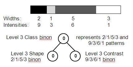
Figure 7: An association of shape and contrast patterns
If other property types were available, such as height from a two dimensional array of sensors or weight from muscle tension, each of these would form a property binon hierarchy. All these types of property binons would then be combined in a lattice to form the class binons.
More sophisticated sensors may provide symbolic values such as book titles or colours. These and other symbolic values are all names for categories of objects. Symbolic values (names) are nominal. They are unordered and come from a set of valid values. Integers can be used to represent them provided no arithmetic operations are performed on them. When a stimulus consists of symbolic values they are represented and stored as integers in level 1 binons and no ratios are calculated. Level 2 and higher binons then combine these categories. For example, if a stimulus was an ordered list of part names such as handle, hammer head, nail, and board, these would be found as integers in level 1 binons. Because handle and hammer head are adjacent their combination would match the level 2 target binon representing the category “hammers”.
A class name such as gizmo is a symbolic value. A name binon is created to represent it. This is then associated with the binons found during the processing of the stimulus, as in Figure 8.
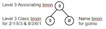
Figure 8: A class binon associated with its class name
The integer value G in the name binon is nominal and represents the symbolic value of gizmo. Name binons can be associated with both property and class binons at all levels. This provides for the categorization of shapes independent of their contrast patterns and vice versa.
Pattern classification is the task of predicting the class name for a given stimulus before being given its correct category. A binon that is not associated with a name binon has not been classified and cannot be used to predict the category. A binon that is associated with one name binon is unambiguous and can be used for prediction. However, a binon that is associated with two or more name binons is ambiguous and is less useful for prediction purposes.
Like all software, Perceptra consists of an algorithm and data structures. The data structures consist of the stimulus, the growing binon network and an activation tree. A new activation tree is created each time a stimulus is processed. This is Perceptra’s short-term memory. The leaves of the activation tree contain the logarithmic values of the sensor readings and any property values derived from them such as width. Higher in the activation tree there are references to the binons that represent the categories found in the stimulus as the features are combined and recognized or created.
To learn efficiently, Perceptra applies two simple rules. First, it only combines two source binons into a target binon when they occur in the same stimulus. This is effectively learning based on coincidence and novelty (Gatsoulis, Kerr, Condell, Siddique, & McGinnity, 2010). This is the same principle underlying the Hebbian learning rule which is often stated as “Cells that fire together, wire together” (Frégnac, 1995). Hebb’s first rule concerning the temporal coincidence or correlation of pre- and post-synaptic firing is most frequently quoted. However, it is his second law that is relevant here. He wrote: “any two cells or systems of cells that are repeatedly active at the same time will tend to become 'associated,' so that activity in one facilitates activity in the other. ... [Here] what I am proposing is a possible basis of association of two afferent fibers of the same order - in principle, a sensori-sensory association” (Hebb, 1949, p.70).
Second, Perceptra uses a simple policy to avoid the combinatorial explosion that would result from the creation of all the binons that represent each stimulus at all the possible levels of complexity. Two source binons must be familiar, that is they must already exist from the processing of a previous stimulus, before they can be combined in the creation of a target binon. This slows down the creation of new binons. Only known patterns are re-used.
Perceptra processes each stimulus into an activation tree, finds existing binons or creates new ones, predicts the object’s category based on past knowledge and finally associates the found and newly created binons with the correct name binon, if provided. Starting with an empty network the steps in more detail are:
1. For each stimulus
1.1. Create the leaf activation tree entries for each part.
1.2. Find existing or create new level 1 binons from the relative values of adjacent parts in the stimulus.
1.3. At each level use the learning rules to combine familiar source binons or create new ones.
1.3.1. Find existing property binons or create new ones as in Figures 5 and 6.
1.3.2. Find existing class binons or create new ones by combining property binons as in Figure 7.
1.4. Predict the category based on the most frequently occurring name binon associated with found unambiguous binons.
1.5. Associate all the found and new binons with the name binon, if provided, as in Figure 8.
In step 1.4, only known unambiguous binons are used for predicting the category of a stimulus. This is done before associating the correct class name in step 1.5. If no class name is provided with a stimulus, step 1.5 is not done but new binons may still be formed in step 1.3. This is unsupervised learning. These categories may be recognized and classified later as stimuli with class names are processed. This is known as semi-supervised learning.
Partially obscured objects can be identified in step 1.4 because there may be many unambiguous class binons that represent different groupings of the sub-categories making up a named category.
Perceptra’s performance was evaluated in the recognition of handwritten digits obtained from the UCI Machine Learning Repository. The original digits, in a 32x32 bitmap, were divided into non-overlapping blocks of 4x4 and the number of “on” pixels were counted in each block. This generated an input matrix of 8x8, where each element is an integer in the range zero to 15. Examples are shown in the first row of Figure 9. This reduced dimensionality but as can be seen that it seriously blurred the images. For Perceptra’s purposes the 8x8 images were transformed back into bitmaps. A threshold of seven or greater for “on” values was used (second row in Figure 9). These images and bitmaps were then horizontally rasterized onto a one dimensional array of 64 sensors.
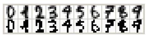
Figure 9: Example 8x8 UCI images and bitmaps
When Perceptra is used to recognize the images in the first row it reaches about a 65% success recognition rate. When recognizing the second row of bitmap digits it reaches more than an 80% success rate as shown in Figure 10.
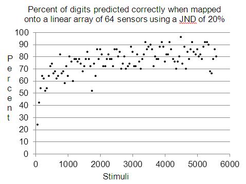
Figure 10: Prediction success rate
In the figure, there is a point for each successive 50 stimuli of the 5600 digits. At the end of the process 45,137 shape binons were created, as shown in Figure 11. The distribution of binons per level peaked at level 6 with 9,394 shape binons. The most frequently used level for prediction purposes was level 8 with a 78% success rate. At higher levels, such as level 12, there were fewer binons. At this level, 455 binons were created and 88 predictions were made of which 96% were correct.
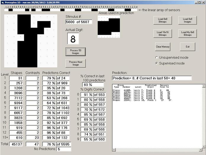
Figure 11: Final screen shot after processing 5600 handwritten digits in supervised mode
When Perceptra is recognizing the bitmapped digits in the second row, contrast is purely black and white. Thus the recognition is taking place primarily based on shape and not contrast. This is most likely the reason for the 15% difference in success rates between the two rows.
Perceptra still needs to be tested on a wider variety of tasks. Even though every binon is a unique category, the large number of binons created needs to be addressed. On larger datasets a pruning strategy may be necessary.
A binon appears to be an AND gate. However, it recognizes the pattern 1/2 as different from 2/1 because of the ordering of the links to source binons. Therefore recognizing rotations, reflections and inversions is not built-in to Perceptra. Similarly humans have to learn through practice that rotated shapes belong to the same or different categories. For example, we have to learn that the letter F is the same letter upside down or backwards but the letter b is different. When upside down, it’s the letter p, and when it is backwards, it’s the letter d.
Binons in a binon network represent categories of objects as combinations of their features. As such they provide for a possible implementation of the perceptual schemata in schema theory (Arbib, 1995), Fuster’s cognits (Fuster, 2003), Barsalou’s perceptual symbols (Barsalou 1999) and category prototypes in prototype theory (Lehrer, 1989).
Like SUSTAIN, Perceptra begins small and expands. It performs incremental implicit category learning and adds categories when surprised by prediction errors in supervised mode. Binons are combinations of features and are equivalent to SUSTAIN’s category clusters / prototypes. However, Perceptra does not resort to probabilistic based approaches. It also lacks a selective attention mechanism as in SUSTAIN.
As in deep learning architectures, such as convolutional networks, Perceptra reuses and shares lower level representations multiple times in the formation of higher level categories. However, unlike convolutional networks, even the lowest level binons are position independent categories.
The use of composition and the subtraction of logarithmic values may be a more plausible explanation of how biological neurons achieve perception than the current emphasis of using weights on links to correspond to the strength of synaptic connections. Composition of source neurons may correspond to the summation of excitatory synapses and the subtraction operation may correspond to the influence of inhibitory synapses. If this is true then the structural configuration of our neurons should play a more prominent role in how we recognize objects.
One of the driving principles used in the design of Perceptra has been Occam’s Razor. The goal has always been to find simpler working explanations. Thus, it is built using a simple component in a simple structure. A binary node is the simplest structural component that can be used to create a hierarchy. This allows networks of binons to scale well across multiple levels of abstraction while also being able to represent any possible configuration or complex combination of features.
The binon network is a deterministic structure. There is no stochastic, probability or statistical inference involved. Thus, there is a direct explanatory relationship between the categories and how they represent the real world.
The resulting system is multi-modal because property types from different senses can be combined using the same principles. Also the stimuli can consist of either graduated or symbolic values.
The power of a compositional hierarchy of categories and very simple mathematics, logarithms and subtraction, are sufficient to perform implicit category learning.
Key Features
Simple
- No stochastic inference
- No back-propagation, feed-forward only
- A one dimensional array of dependent sensors
Grounded
- Graduated (ratio scale / numeric) and/or Symbolic (nominal) input
Deterministic
- A direct explanatory relationship to the real world
- No hidden layers
Supervised and/or Unsupervised
- Continuously adaptable
Multimodal
- Multiple properties / features / dimensions
Avoids the combinatorial explosion
- Economical
- - Grows when needed
- - Only ratios with a just noticeable difference are kept
- Common patterns / categories are shared
Scales well
- Recognizes obscured objects
Recognition independent of:
- Position
- Size
- Intensity level
- Order of magnitude of intensity
No built-in recognition of:
- Rotation
- Reflection
- Inversion
Neurological plausibility
- Grounded on sensory data
- Grows bottom-up
- Hierarchical structure
Other versions of Perceptra:
- 2D - classifies patterns using a two dimensional array of sensors
- Independent - classifies patterns using independent sensors / senses, such as the joint angles of limbs with multiple degrees of freedom
Arbib, M. A. (1995). Schema theory. In M. A. Arbib (Ed.), The Handbook of Brain Theory and Neural Networks. Cambridge, Massachusetts: MIT Press.
Barnden, J. A., Y. (1995). Semantic networks. In M. A. Arbib (Ed.), The Handbook of Brain Theory and Neural Networks. Cambridge, Massachusetts: MIT Press.
Barsalou, L.W., (1999). Perceptual symbol systems. Behavioral and Brain Sciences, 22, 577–660
Bengio, Y. (2009). Learning deep architectures for AI. Foundations and Trends in Machine learning, 2(1), 1-127
Bienenstock, E. & Geman S. (1995). Compositionality in Neural Systems. In M. A. Arbib (Ed.), The Handbook of Brain Theory and Neural Networks. Cambridge, Massachusetts: MIT Press.
Cesa-Bianchi, N., Gentile C., & Zaniboni L. (2006) Hierarchical classification: combining Bayes with SVM. Proceedings of the 23rd International Conference on Machine Learning (pp. 177-184). Volume 148 of ACM International Conference Proceeding Series, ACM.
Chaudhary, V., Ahlawat, A.K. & Bhatia, R.S. (2011). Growing Neural Networks using Soft Competitive Learning. International Journal of Computer Applications, 21(3).
Dickinson, S. (2009). The evolution of object categorization and the challenge of image abstraction. In S. Dickinson, A. Leonardis, B. Schiele & M. Tarr (Eds.), Object Categorization: Computer and Human Vision Perspectives. New York: Cambridge University Press.
Fahlman, S. E. & Lebiere, C., (1990). The Cascade-Correlation Learning Architecture. Advances in neural information processing systems, 2, 524-532
Fechner, G.T. (1966). Elements of psychophysics (Vol. 1) E.G. Boring & D.H. Howes (Eds.); H.E. Adler, (Trans.). New York: Holt, Reinhart & Winston. (Originally published in 1860)
Fidler, S., Boben, M. & Leonardis, A. (2009) Learning Hierarchical Compositional Representations of Object Structure. In S. Dickinson, A. Leonardis, B. Schiele & M. Tarr (Eds.), Object Categorization: Computer and Human Vision Perspectives. New York: Cambridge University Press.
Frégnac, Y. (1995). Hebbian synaptic plasticity: comparative and developmental aspects. In M. A. Arbib (Ed.), The Handbook of Brain Theory and Neural Networks. Cambridge, Massachusetts: MIT Press.
Fukushima, K. (1988). Neocognitron: a hierarchical neural network capable of visual pattern recognition. Neural Networks, 1(2), 119-130.
Fuster, J. M. (2003). Cortex and Mind. New York, NY: Oxford University Press.
Gatsoulis, Y., Kerr, E., Condell, J. V., Siddique, N. H. & McGinnity, T. M. (2010). Novelty detection for cumulative learning. Proceedings of Towards Autonomous Robotic Systems 2010 (pp. 62-67). Plymouth, UK: University of Plymouth.
Hebb, D.O. (1949). The Organization of Behavior. New York, John Wiley & Sons.
Hummel, J.E. & Biederman, I. (1992) Dynamic binding in a neural network for shape recognition. Psychological Review, 99(3), 480-517.
Hummel, J.E., Holyoak, K.J., Green, C. et al (2004) A solution to the binding problem for compositional connectionism. In S.D. Levy & R. Gayler (Eds.), Compositional Connectionism in Cognitive Science: Papers from the AAAI fall symposium, (pp. 31-34). Menlo Park, CA: AAAI Press.
Jlassi, C., Arous, N., & Ellouze N. (2010) Phoneme recognition by means of a growing hierarchical recurrent self-organizing model based on locally adapting neighborhood radii. Cognitive Computation, 2(3),142-150.
Kohonen T., (1998). The self-organizing map. Neurocomputing, 21(1–3), 1–6.
LeCun, Y. (2012). Learning invariant feature hierarchies. European Conference on Computer Vision (ECCV 2012), (pp. 496-505). Lecture Notes in Computer Science, Springer-Verlag Berlin Heidelberg, Workshop on Biological and Computer Vision Interfaces.
LeCun, Y., Bottou L., Bengio, Y., and Haffner, P. (1998) Gradient-based learning applied to document recognition. Proceedings of the IEEE, Vol. 86(11), 2278–2324
Lehrer, A., (1989). Prototype theory and its implications for lexical analysis. In S. L. Tsohatzidis (Ed.), Meanings and Prototypes: Studies in Linguistic Categorization. London: Routledge.
Love, B.C., Medin, D.L. & Gureckis, T.M. (2004). SUSTAIN: A Network Model of Category Learning. Psychological Review, 111(2), 309-332.
Portugal R. D., & Svaiter B. F. (2011) Weber-Fechner law and the optimality of the logarithmic scale. Minds and Machines, 12(1), 73-81.
Sharma, S. K., & Chandra, P. (2010). Constructive neural networks: a review. International Journal of Engineering Science and Technology, Vol. 2(12), 7847-7855
Starzyk, J. A., He H., & Li, Y. (2007). A hierarchical self-organizing associative memory for machine learning. Lecture Notes in Computer Science 4491: 413-423.
Weber, E. H. (1850). Der Tastsinn und das Gemeingefuhl. In Handwörterbuch der Physiologie, Vol. 3. Braunschweig.
This paper can be downloaded from the following link:
Martensen, B. N. (2013). Perceptra: A New Approach to Pattern Classification Using a Growing Network of Binary Neurons (Binons). In R. West & T. Stewart (eds.), Proceedings of the 12th International Conference on Cognitive Modeling, Ottawa: Carleton University.