
2012 Incomplete patent application
Software Patent Application 20th November 2012 (c) 2012, Adaptron Inc.
Pattern Classification using a Growing Network of Binary Neurons (Binons)
Executive Summary
This document describes a software application that can be used to recognize objects. Typical uses would be in image or speech recognition. The software learns about the real world by experiencing it through sensors. It builds up an artificial neural network of its knowledge as a long-term memory and uses this to identify things that it has not previously perceived.
Table of Contents
Abstract
Introduction
Background
Fundamentals
Principles of Operation.
Patterns of Relationships
Aggregation Rule
Weber-Fechner Law
Synchronicity
Requirements
The Classification Process
The Binon Network Data Structure
Level-1 Binons
Level-2 Binons
Level-3 Plus Binons
The Activation List
The Recognition Algorithm
Algorithm Features
How Perceptra learns
Other Approaches
Applications of Perceptra
Images
Sounds
Data
Future Applications
Motor Control
Perceptual Grouping
References
Convolutional Networks
Deep Learning
Novelty detection
Constructive Pattern Recognition
Hierarchical and relational structures
Object Categorization of Images
Relationships
Other Patents
Abstract
General-purpose pattern classification must identify classes of objects independent of the absolute values of their properties. Such properties include position, size, orientation, intensity, reflection, inversion (negative) and level of complexity. Properties that are invariant for objects of the same class include their shape and contrast patterns. Shape is the relationship between the sizes of an object’s parts and contrast is the relationship between the intensity of its parts. A binon is a binary neuron that records the relationship between two source binons. A hierarchical network of binons is a practical structure for representing these relationship patterns. With a classification algorithm transforming an array of sensory readings into relative property values, both familiar and novel objects can be learned and identified without the need to introduce weights on interconnections or use statistical inference.
Introduction
This document describes the requirements, solution and application of a general-purpose pattern classification algorithm (Perceptra) that can be used in any software system that needs to perform class or object identification.
Wherever alternate terminology exists for the same concept this is found in curly brackets following the term used in this document. Important terms are underlined where they first appear or are defined.
Background
Pattern classification software is used in any system that needs to identify classes or objects from a set of input properties {data or feature set}. Examples of such systems are:
- Handwriting recognition for addresses on envelopes,
- Facial recognition for identifying people entering a bank,
- Recognizing types of trees in a forest,
- Speech recognition of voice commands to a smart phone,
- Optical character recognition of documents,
- Sound recognition to identify birds by their songs and
- Motion recognition by an autonomous robot to control its actions.
There are many different classification algorithms used for pattern classification. Some common pattern classification techniques use:
- Statistical inference algorithms based on probabilities,
- Shape extraction algorithms based on grouping of related features,
- Non probabilistic mathematical algorithms that manipulate the input data, and
- Syntactic {structural} algorithms that use strings or graphs.
Statistical inference algorithms based on probabilities are used in artificial neural networks (ANNs). In this approach the structure is composed of many layers of neurons {nodes}. The first layer is used for input of the data to be recognized and classified. The last layer has neurons for each class or object that must be identified. There are multiple links between neurons of adjacent layers. The links between the neurons have weights. An activation algorithm sums the weights of the incoming links to determine the activation of each node. In feed forward ANNs activation flows from the input to the output layer of neurons via the intermediate neurons called hidden layers. In recurrent ANNs feedback information is used and it flows in the opposite direction.
Shape extraction algorithms based on the grouping of features are usually used in visual object recognition {object categorization}. In this approach, specific features such as edges, corners and primitive shapes are found in the image. Classes of objects are then identified based on the grouping of related or adjacent features. Features are hand crafted by the designer for this purpose.
Non probabilistic mathematical algorithms that manipulate data are used to generate clusters of similar data. The clusters are formed in a multi-dimensional space. These clusters represent classes {categories} of objects. This is done without any specific label being attached to the category in advance. See unsupervised learning below.
Syntactic {structural} algorithms use strings or graphs to capture relationships between the input values. The grammars for the recognizable strings or the prototypes for the graphs are specified by the algorithm designer. This approach is only used where the data can be represented symbolically {discretely} (without any numerical values)
Pattern classification algorithms learn the identity {label or name} of their output classes and objects by using a Supervised, Unsupervised, Semi-supervised, or Reinforcement learning approach.
- Supervised learning trains the algorithm on a set of values {exemplars} which have been labelled with the correct names for the classes or object. After training it is used to recognize the same classes or objects but from different sets of input values. Further training is not performed.
- Unsupervised learning categorises input values into clusters of similarity without any training, labels or feedback information. This approach works continuously to identify new clusters of similar data which presumably are for objects of the same class.
- Semi-supervised learning is a combination of supervised and unsupervised learning in which a subset of the input values has been labelled correctly. This reduces the work required to have a sufficiently large set of labelled data for training purposes. It also associates class and object names to the clusters for identification purposes.
- Reinforcement learning trains unsupervised learning algorithms with feedback {reward} for correct classification without explicitly identifying the class or object.
Fundamentals
Pattern classification {object categorization} is a subset of pattern recognition. Pattern recognition is a machine learning process. Pattern recognition also includes regression analysis and sequence learning. Regression analysis is the assignment of real-valued outputs to a set of input properties. Sequence labelling is the assignment of a class to each member of a sequence of values ordered in time.
The fundamental concepts that apply to pattern classification are illustrated in Figure 1 and described below.
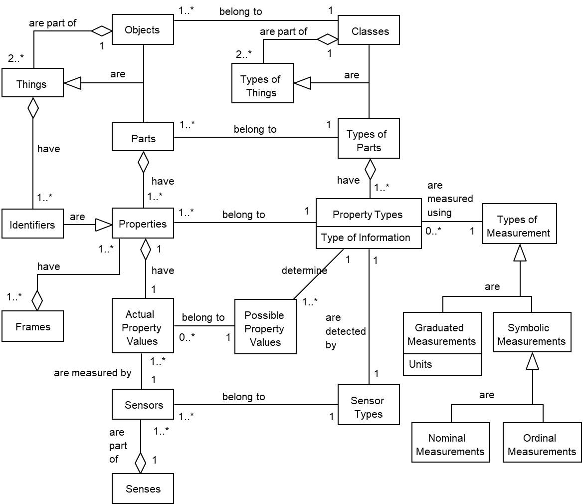
Figure 1. Fundamental concepts
Pattern classification identifies {labels, names} a class {type of thing, category or kind of thing} or an object {thing or instance of a class} based on its properties. "Hammer" and “tool” are examples of classes while "my hammer" is an object. The smallest possible object is a part. It is indivisible or has no sub-parts. Objects are composed of parts. Parts have properties {features, attributes, or characteristics}. My hammer is composed of its head and handle. Its head has the property of weighing 550 grams. Every property belongs to a property type. For my hammer the property type is weight. Each property type corresponds to a different type of information, has a set of possible values and is measured using a particular type of measurement. Other examples of property types are colour, size, temperature, and priority. The possible values for colour could be red, yellow, green and white. Properties also have actual property values {measurements, settings or readings}.
Classes and objects have a unique identifying property {label or name}. For example all apples belong to the class named "apple". But classes and objects may also have non-identifying properties. For example all apples have the common properties of shape equals round and biological equals true. And my apple has the specific values for its properties of colour equals red, weight equals 101 grams, and height equals 9.3 centimetres. Pattern classification must learn the association between patterns of non-identifying properties and the identifying ones. A subset of an object's properties determines its class while all of its properties are necessary to determine which object it is. In this respect classes and objects form a continuum in which objects are the most specialized and classes are more general. An object may belong to many classes. For example, the cat with object name "Fluffy" belongs to the class "cat" that belongs to the class "feline" that belongs to "mammal" and then "animal" etc.
Types of measurement {levels of measurement} are based on the interdependency of the possible property values for a property type. Two types of measurement for values are symbolic and graduated.
- Symbolic {discrete, qualitative or categorical} property values are divided into two types: nominal and ordinal.
Nominal values are independent of each other because they have no inherent order. They come from an unordered set. Examples are the colour property values: red, blue, brown, green, and white and the fruit type names: apple, orange, pear and banana. Class and object identifying values are nominal.
Ordinal values are dependent on each other because they are inherently ordered. Therefore they form a list. A list of values can always be represented by {mapped onto} a set of integers. But when values are ordinal no arithmetic can be performed on them. For example the values may be ordered alphabetically or be in some conceptual order such as High, Medium and Low.
- Graduated property values {intensities} are those that can be represented by real valued numbers. They are inherently ordered. Real valued numbers can only be represented to a certain number of decimal places {resolution or degree of accuracy}. This means they can be mapped onto a set of integers. Unlike ordinal values, arithmetic operations can be performed on them. Graduated property values have units of measurement that correspond to the type of information of the property. For example gram units for weight and decibel units for volume.
Each set of input properties that needs to be recognized is called a frame {instance, exemplar or example}. The property types and structure of the properties in a frame depend on a sense, its sensor types and their configuration.
A sense is a mechanism for gathering information about the world. Each sense detects a form of energy. For example sight detects light and hearing detects sound. Senses are always independent of each other. A sense is made up of sensors. A sensor {receptor cell, detector} is a device that detects a particular kind of energy and provides a measure of its intensity. This measure is an actual property value. Sensor types are based on the type of property they measure. Two examples of symbolic value sensors: one that measures blood types and one that scans a book and provides the title. Three examples of graduated value sensors: a sound sensor that measures volume, a light sensor that measures brightness and a joint sensor that measures angle. A sense may have one or more sensor types. For example the sense of sight has brightness and colour sensors while the sense of smell only has aroma sensors.
A frame contains a sense's set of property values that need to be recognized and a list of identifying data items. The property value set is divided into one or more subsets based on the sense's sensor types. For example for the sense of touch there may be sensors that are detecting pressure (texture), temperature and state (gas, liquid or solid).The list of identifying data items contains the names for the classes and / or object corresponding to the property values. In lifelong learning the pattern classification process cycles through the steps:
- Analyse the relationships and dependencies between the values in a frame.
- Predict the classes and / or object for the frame based on past experience.
- Use the correct classes and / or object identifiers to update the experience.
Within each subset of values, determined by the sensor type, there may be one or more sensors providing property values. Values from these sensors may be ordered or unordered depending on the configuration of the sensors. Dependent sensors {linear, one-dimensional, or contiguous} provide an ordered list of property values. They are dependent on each other {related} because they are adjacent. For example touch sensors are adjacent to each other. Position is determined by the position of the sensor in the list. If there is more than one sensor type at a given position multiple values are detected per position. Independent sensors provide property values that are unordered and independent of each other {unrelated}. Independent sensors can be thought of as all adjacent to each other. For example joint angle sensors are independent because the sections of our limbs can be moved independently. The same is true for rotational position sensors of motors controlling robot limbs or wheels.
In pattern classification the identifying values are symbolic. However if these values are graduated then the process is performing regression analysis.
Time is also a dimension that can be measured. When frames have a temporal order a pattern classification algorithm performs what is called sequence labelling. The timing of the frames is a graduated property value. When time is not involved a pattern classification algorithm learns independently of the order in which the frames occur.
Principles of Operation
Patterns of Relationships
If one has a single property value from a single sensor then one has a measure of a property for a single part. The resolution of the sensors determines the smallest part that can be detected. But the property value from a sensor does not necessarily identify the part so that it can be re-identified later. A graduated property value such as the volume from a given frequency sensor does not identify the sound. The same sound may occur again at a different volume. However a symbolic value from a given sensor does identify a part. Examples include: a sensor that returns the title of a book, one that identifies your gender or one that recognizes the chord played on a piano.
For graduated property values more than one sensor's value is needed to identify a part. However, in the case of dependent sensors two or more adjacent sensors may be measuring the property value of the same part of an object. In this case the two values will be the same and the part cannot be identified. On the other hand if two adjacent values are different, then the sensors must be detecting separate parts of the same object. The ratio of these two values will not change as the object moves or changes in intensity and therefore the ratio can be used to identify the smallest detectable part.
In general the principle for uniquely identifying an object when dealing with graduated property values is based upon:
- An object is composed of its parts and
- The relationships between the property values of its parts are constant even if the total value of the property for the object is different.
The relationships between the parts form a property type pattern and the pattern is what identifies the class or object. Relationships are represented as ratios and ratios are calculated using division. A pattern is the aggregation of {combination of, composition of, built out of, made up of, sum of or integral of} these ratios.
Consider size as an example of a graduated value. Size is an important property because a pattern of two or more sizes determines a shape. The size {width} of a part will be the count of the adjacent sensors that are detecting the same value. In order to identify a shape independent of its position and total size it must be recognized based on the relative sizes {ratio of sizes} of its parts. This relationship pattern {shape pattern} remains constant for a given object.
Similarly, other patterns of graduated property values, such as intensity or volume, from two or more adjacent sensors determine contrast. An object's contrast is the relative intensity {ratio of values} of its parts. A contrast pattern remains constant for an object independent of its position, size or total intensity.
When a complex object consists of more than one property type (e.g. size, pressure and temperature) the same aggregation approach applies to form the pattern of relationships between the patterns for each property type. The size, pressure and temperature patterns must be aggregated. See the Aggregation Rule below for how this is done. Another example is that both the shape and contrast patterns are needed to identify and distinguish between a filled in black circle and a perfectly circular orange in shades of grey. Shape and contrast patterns are aggregated to more accurately identify a class or object.
For symbolic valued parts the same pattern of relationships principle applies except ratios for contrast are not possible. Also when sensors are unordered they are independent and no concept of size can exist. However the same pattern of sensors and the same pattern of symbolic values must be uniquely identified if they are to be recognized again. Identifying symbols and sensors by assigning them ordinal values supports this. For example three independent sensors measure the three symbolic values B, N and M. In pattern classification it is necessary to recognize the same combination of three symbols independent of which sensors detect them. If the symbols are ordered alphabetically as they are combined only one combination will result, BMN. This is the symbol pattern equivalent to the contrast pattern for graduated values. It is also necessary to recognize the sensor combination on which these three symbols were detected. They may have been detected in any one of the six orders of B, M, and N that are: BMN, BNM, NBM, NMB, MBN or MNB. But to structure these order patterns the sensors must be given an ordinal value - their position. This is the order pattern equivalent to the shape pattern for adjacent sensors.
Table 1 summarizes the different pattern types produced based on the sensors being dependent or independent and their property type values being graduated or symbolic.
- Shape patterns are produced from sizes.
- Contrast patterns are produced from intensities.
- Order patterns are produced from sensor positions.
- Symbol patterns are produced from symbolic values.
| Pattern types based on: | Graduated values | Symbolic values |
| Dependent Sensors | Shape & Contrast | Shape & Symbol |
| Independent Sensors | Order & Contrast | Order & Symbol |
Table 1. Pattern types based on sensor dependency and property type values
Both classes and specific objects can be recognized and identified using the patterns of relationship principle. An object will have a unique set of property patterns. A class however will be associated with many objects. But all objects of a class will contain the same subset of property patterns that identify the class.
If one is performing sequence labelling, one is trying to identify a class or object as it is changing in time. Time then becomes an additional property type and the timing pattern is relevant. The same pattern of relationships principle applies because all the parts of a class or object change in unison and retain their relative values.
Once a class or object has been identified as a result of its shape/order and contrast/symbol patterns other derived properties of the class or object can be determined. If the sensors are ordered then rotation {shape orientation}, which is the order of occurrence of adjacent sizes, can be derived. If the measured values are graduated then some common derived properties are:
- Reflection {contrast orientation} - The order in which adjacent values occur, and
- Inversion {negative/positive} - The reverse pattern of adjacent values.
However these derived properties are learned through association with classes and objects and are not measured. See the Aggregation rule below for an explanation of association.
Aggregation Rule
The aggregation rule determines the process for representing all possible combinations of a given set of parts when using binary nodes in a network data structure. Two parts that are lowest level {terminal or level-1} nodes can be combined into a binary node via two links. The binary node {target node} represents the pair as a single unit.
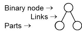
The two parts {source nodes} are now associated with each other via the binary node. Association is therefore defined between two objects when they are linked to a common target node.
Larger combinations of 3 or more parts can be formed with binary nodes and represented as a single node by linking additional nodes from lower levels.
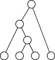 or
or 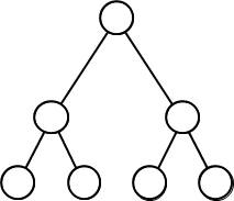
However if a restriction applies that only nodes of the directly lower level can be used as source nodes then the only solution that correctly combines odd and even numbers of nodes requires that there be overlapping sub-nodes.
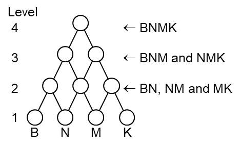
In this example and assuming that the parts are ordered, not all combinations of parts are represented. BM, BK, NK are missing at level-2 and BNK and BMK are missing at level-3. The solution to this is to produce all possible pair combinations at level 2 and then only produce higher level combinations in which the two parts share a common sub-part. For example BMK is the combination of BM and MK and M is the common sub-part. An example at a higher level based on level-1 parts of B, N, M, K, E and A is BNMEA. BNMEA is the combination of BNME and NMEA in which NME is the common sub-part. BNME is the combination of BNM and NME in which NM is the common subpart. For a given list of N ordered parts this algorithm will produce all 2^N -1 combinations if one includes the N parts at level-1 in the count. Since this example is based on a specific ordering for the symbolic values not all possible permutations of the 4 symbols are generated.
In this hierarchical {tree} structure the number of lowest level parts is the same as the levels used and is equal to the level of complexity of the highest level node.
Weber-Fechner Law
E. H. Weber stated that the just-noticeable difference (JND) between two stimuli is proportional to the magnitude of the stimuli. This applies when considering graduated values. For example when one has a weight in each hand it is hard to tell whether the weights are different when they are closer together in actual weight. If one weight is 101 grams and the other 102 grams one cannot tell if they are different. But if one weight is 100 grams and the other 200 grams the difference is easily detected. G. T. Fechner went further by stating that human subjective sensation is proportional to the logarithm of the stimulus intensity. This just-noticeable difference effect can be obtained by using the integer value of the difference between the logarithms of the two stimuli intensities in the calculation of the relationship between them.
For example the relationship between 101 and 102 is the ratio 101/102. Using normal division this ratio would be non-zero and therefore noticeable. However when using integer {truncated} values and the logarithmic rule that Log(A / B) equals Log(A) - Log(B) in any base one gets a result of zero, which is not noticeable.
Perceptra uses integer base 1.2 logarithms {Log1.2}. This means the integer difference in the logarithm values only becomes a non-zero value when the difference is greater than approximately 20%. For a 30% JND use a logarithm base of 1.3.
The base 1.2 logarithm of 101 is 25.31308 and 102 is 25.36712. The difference between these two values is -0.05404. The integer value of this is zero and this difference is not noticeable. However, Log1.2 (100 / 200) equals Log1.2 (100) – Log1.2 (200) which is 25.25850 – 29.06029 = -3.80179 and the integer value of this is -3 which is non-zero and noticeable. By using this rule and the logarithmic formula on the ratios between graduated property values of the same property types, patterns of relationships can be produced with the same just-noticeable difference characteristic. Also the only arithmetic operator required is subtraction.
Logarithms cannot be calculated for zero or negative numbers. So when property values include zero as a valid measurement the value is incremented by 1 before the logarithm is determined.
Synchronicity {contiguity, co-occurrence, coincidence or simultaneous events}
Given many frames of random values {noise} all possible pairs of values will occur due to coincidence. Triplets of the same values will reoccur but less frequently. Larger combinations of values will reoccur but even less often. However the real world contains objects whose property values are not random. Repeatable simultaneous combinations {patterns} of values reoccur more frequently than at random. Although all possible pairs of values probably reoccur in the real world, not all the possible larger combinations reoccur. A structure that records all the real world combinations would therefore have representations of all the smallest combinations but only representations of a subset of all possible more complex combinations. This is the same principle underlying the Hebbian idea that "Cells that fire together, wire together". The coincidence of the cells firing causes them to be connected {associated} in some fashion. It can also be used as the principle supporting reinforcement learning. Co-occurrence of a pattern of values that is novel {unknown} is rewarding while one that is familiar {known} is not rewarding. This is the principle of novelty detection.
Requirements
A general-purpose pattern classification algorithm should satisfy the following requirements.
- Learn to recognize classes and objects independent of the absolute values of their position, size, intensity, orientation, reflection, inversion and level of complexity.
- Continuously classify new patterns and recognize known ones {lifelong learning}.
- Use the simplest possible representation of the classes and objects.
- Recognize an object even though part of it is obscured.
- Work on any type of information that can be measured via sensors.
The Classification Process
Like all software the Perceptra process consists of data structures and an algorithm that uses the data structures. This process builds a permanent and growing lattice network structure of binary neurons {binons} to represent the long-term memory of classes and objects. It also builds a temporary activation list of binary neurons and their measured property values from each frame. The algorithm uses the property values in the activation list to determine the binons. It uses the network of binons to determine whether they are familiar or novel. It then predicts and / or updates the associated classification in the binon network.
The Binon Network Data Structure
Perceptra builds an artificial neural network of binary neurons called binons. A binon network is designed to represent the pattern of relationships {ratios, relative properties, differences, changes, or derivatives} between the values of the parts that comprise a class or an object. A binon has two ordered links {connections}, each to a lower level source binon. But as a source neuron a binon may be linked to many other higher-level target binons - Figure 2. The result is a lattice network {heterarchy}. Via its links each binon is an aggregation of and thus represents the combination of the two source binons. It captures the principle that an object is made up of parts.
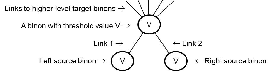
Figure 2. A binon and its links to two source binons
There are several types of binons based on their level in the network and the purpose they serve.
- Level-1 binons – represent the values or parts detected by sensors.
- Level-2 binons – represent the relationships between level-1 binons.
- Level-3 plus binons – indirectly represent a pattern of three or more level-1 binons by being combinations of level-2 or level-3 plus binons.
The links do not have weights as are found in normal multi-level {multi-layer} artificial neural networks. However each binon has an optional integer threshold value V. The threshold value serves different purposes depending on the level of the binon in the network structure and the property type of the sensors. At level 1 a threshold value represents a symbolic value or is set to zero for graduated sensors. At level 2 it represents the ratio between two sensor values if they are graduated and is irrelevant and set to zero if values are symbolic. At level 3 and higher the threshold is not relevant and is set to zero.
As illustrated in Figure 3 at all levels there are two types of binons: property and object binons. Property binons represent a pattern of values from the same property type. Object binons are aggregations of property binons at the same level.
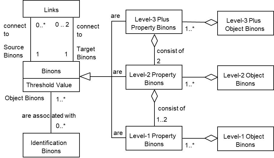
Figure 3. The Binon Network Structure
Level-1 Binons
Level-1 binons are not linked to sensors. For symbolic values level-1 binons represent and identify the smallest possible recognizable parts. For graduated values there is only one level-1 binon per property type. Graduated values are not kept in level-1 binon thresholds. See Figure 4 below.
Level-1 property binons
The two links of a level-1 property binon are not connected to any nodes and are set to null. For sensor values that are symbolic, level-1 threshold values of property binons represent the symbolic values. See Figure 5 below. For graduated values level-1 binon threshold values are set to zero. See Figure 4 below.
At least two level-1 property binons are identified per sensor position.
- For dependent sensors one is always the size binon and the others are for the symbolic values measured by the sensors at the position or for the property types measured at the position. Size is a graduated value. A single sensor position has a size of one. Size is only greater than one when two or more adjacent sensors produce the same measured value and are combined. This happens when they are detecting the same part of a real world object.
- For independent sensors one is always the sensor position and the others are for the symbolic values measured by the sensors at the position or for the property types measured at the position.
Level-1 object binons
The level-1 property binons are combined according to the aggregation rule to form level-1 object binons. An example would be the combination of size and intensity. But note that both of these are graduated values and therefore this level-1 object binon does not identify a part. However if at least one of the property binons is symbolic a part is identified. An example is a chord and a volume. All level-1 object binons have a threshold value set to zero.
Identification binons are level-1 symbolic valued object binons for the classes and / or object names given as the identifying data items for a frame.
Level-2 Binons
Level-2 property binons
If the property values are symbolic then a level-2 property binon has 2 links to level-1 property binons of the same property type and its threshold is zero. See Figure 5 below. In this case the level-2 binon represents the coincidental occurrence of the two symbolic values. Thus the level-2 binon represents a pattern. The two links and their source binons are ordered. A symbol pattern has the source binons ordered according to sensor position if sensors are dependent and according to symbolic values if sensors are independent. For independent sensors an order pattern has the source binons ordered according to the order of the two sensor positions.
If the property values are graduated then each level-2 property binon has 2 links to the same source level-1 binon. The level-2 binon's threshold value is the integer difference between the Log1.2 values of the two source sensor values calculated as in the Weber-Fechner Law principle. The order of sensor positions is used for contrast and shape pattern calculations.
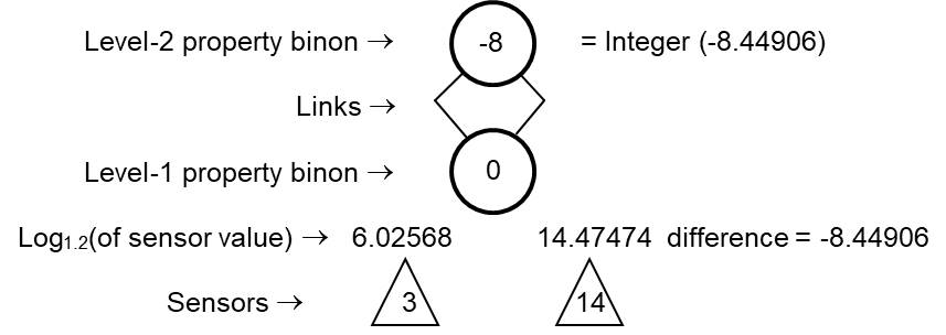
Figure 4. A Level-2 graduated property binon example with dependent sensors
Figure 4 is a graduated value example: The first sensor’s value is 3 and the second sensor’s value is 14. The two sensors used are the ones with value 6.02568 = Log1.2(3) and 14.47474 = Log1.2(14) respectively. The level-2 property binon has two links to the same level-1 binon for the property. The level-2 property binon now represents the ratio of 3 to 14 based on the integer difference of the logarithms. This level-2 property binon represents the 3/14 ratio and any multiple of these such as 6/28. But because the integer value of the difference in logarithms is being used it also represents any ratios within about plus or minus 10% of 3/14. The ratios of 3/13 and 3/15 will also produce a -8 integer value from the difference in logarithms.
Level-2 object binons
The two or more level-2 property binons available per sensor position are combined according to the aggregation rule to form level-2 object binons with threshold values of zero.
Level-3 Plus Binons
There are level-3 plus property and object binons as in level-2 binons. Level-3 plus binons are symbolic in their representation of patterns and need no threshold values. Their representation comes purely from the ordered links they have to their two source binons.
Level-3 Plus property binons
The two source property binons of a level-3 plus property binon are two level-2 property binons or two level-3 plus property binons of the same property type. Combinations of source property binons in a level-3 plus property binon follow the aggregation rule. This means the two source binons must link to a common sub-source binon {overlap}. This allows a level-3 plus property binon to represent a pattern of three or more property values. Figure 5 illustrates this for a level-3 plus property binon. At this level of complexity the overlap is for one level-1 property binon. In general, at level of complexity equal to N the overlap is a level-(N-2) property binon. In this figure the letters B, N and M have been placed in the level-1 binons for illustration purposes only. In the actual data structure integer values based on the symbolic values would be in these binons.
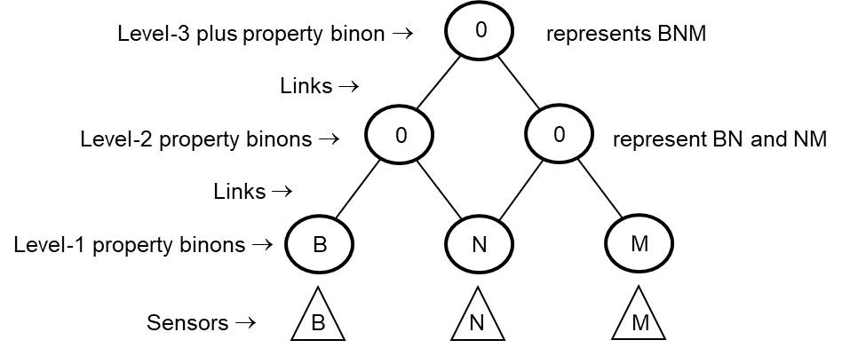
Figure 5. A Level-3 plus symbolic property binon example with dependent sensors
Level-3 plus object binons
Level-3 plus object binons are aggregations of two or more level-3 plus property binons at the same level of complexity but from different property types as sources. The threshold values are not important and are set to zero.
The Activation List
The activation list contains the property values from the frame and the objects recognized and / or created. As the recognition algorithm processes these sensor property values it identifies parts and objects based on relationships between the values. The parts and objects identified are found in the binon network if they are familiar or added to the network if they are novel. As a result each entry in the activation list contains the identity of a novel or recognized property or object binon. It also contains the values for the object (e.g. size) depending on the type of properties and type of binon involved. The activation list is recreated from scratch for each frame when frames have no temporal order. If a temporal order exists between the frames then there are two activation lists, one for the current frame and one for the previous frame.
Activation list entries are added in layers as each level of binons is created for the given frame. If a list entry is for a property binon it will contain:
- The sensor position,
- Property type,
- Property value,
- Logarithm of property value if graduated
- The binon identity,
- And pointers to the two lower layer activation list entries, if any, that contain the source information that was aggregated.
If a list entry is for an object binon it will contain:
- The sensor position,
- The binon identity,
- And pointers to the two property or aggregation binon list entries in the same layer that contain the source information that was aggregated.
The Recognition Algorithm
In this algorithm the term "identify a binon" refers to the process:
- Try to find a binon in the binon network
- If it is not found then
- Create and add it to the network and mark it as novel
- Add the binon to the activation list with the additional information required.
The term "aggregate" is used to refer to the process of combining source binons and building a structure as described in the Aggregation Rule.
To find a binon in the network the four values needed are:
- the two source binons in the given order,
- the property type and
- the integer threshold value.
Binons are never deleted from the network.
The Perceptra process of using the binon network and activation list in pattern classification consists of the steps:
- Start with an empty Binon Network
- Process a Frame - For each frame of values:
- Start with an empty activation list
- Generate level-1 object binons - For each sensor position:
- If the sensors are dependent then
- Identify the level-1 size binon and use the Log1.2 value of the size, which is the sensor's size (equals one for a single sensor)
- If the property type is graduated then
- For each sensor property type, at this sensor position, use its property type and intensity to identify the level-1 property binon and a log value equal to the Log1.2 value of the sensor's reading.
- Else if the property type is symbolic then
- For each sensor property type, at this sensor position, use its property type and reading to identify the level-1 property binon.
- Aggregate the level-1 size, if it was identified and the other property binons to identify the level-1 object binon for this sensor position.
- If the sensors are dependent then
- Treat level-1 as the source level for performing the next steps.
- Generate higher level object binons - For each pair of adjacent source level activation list entries repeat the following steps while they continue to identify at least one known object binon
- Combine adjacent objects that are the same - If the sensors are dependent and two or more adjacent source level object binons are the same then combine the two or more activation list entries using the same object binon at this source level but change the size to the number of sensors spanned by the same object binon.
- If the source level property binons are both familiar then
- Aggregate the source level shape or order and property binons and identify the target level (equals the source level + 1) shape or order and property binons.
- Aggregate the target level shape or order and property binons to identify the target level object binons.
- Treat this target level as the source level.
- 2.5 Predict the classes and / or object recognized - Find the highest-level familiar object binon with the fewest links to target binons. Novel binons will have no links to target binons. Find the associated identification binons and report these as the expected / predicted classes and / or object
- 2.6 Learn the correct classes and / or object - Identify level-1 symbolic valued object binons for the classes and / or object names given as the identifying data items for the frame. These are the identification binons.
- For all the familiar object binons in the activation list
- If there are any identification binons that are not already associated with this object binon then
- Remove all associations between this object binon and its identification binons
- If there are any identification binons that are not already associated with this object binon then
- For all the novel object binons in the activation list
- Identify associating binons that associate this object binon with the identification binons.
- Change the object binon’s status from novel to familiar
Algorithm Features
Identification binons are only associated with the object binons. Lower level object binons in the binon network structure will re-occur in multiple frames and end up being common patterns that are found in multiple classes and objects. When this happens, the algorithm removes the associations between familiar object binons and their identification binons. These object binons are not useful for object identification. However the highest-level familiar object binon associated with class and /or object identifying binons will be the largest subset of parts that are known to uniquely identify the associated classes and / or object. This will be the best prediction of the classes and / or object based on past experience.
The lowest-level familiar object binon with one or more links to target associating binons will be the smallest subset of parts that are known to uniquely identify the associated classes and / or object. This determines the minimum set of parts that are required to recognize a class or object that is partly obscured.
Only familiar source level property binons are aggregated to identify target level property binons. Thus as soon as a property binon is novel for the frame it is no longer aggregated with other same level property binons. Thus only one level of novel binons can be added to the network per frame experienced. Note that novel binons remain novel during the analysis of a frame and only have their status changed to familiar at the end of each frame.
Classes and objects are recognized independent of their sensor position, size, and property intensity because these values are not kept in the binon network structure.
Binons are dependent on the order of their source binons and thus reflections, orientations and inversions produce different binons. This means that recognizing these different objects is only possible by association with classes or objects. This is what we experience. As an example we must learn to recognize letters that are reflections or upside down as the same letter. This is why we must learn to read words upside down; they are not immediately recognized once we have learned them in the upright format. Most upper and lower case letters are the same in their reflected and upside down versions and once learned are easily recognized. However the lower case letters b, d and p are reflections or orientations of each other. The extra effort required in reading reflected or upside down words, containing these letters, illustrate the learning involved.
How Perceptra learns
Perceptra uses reinforcement learning based on novelty detection to form its object binons. This means that if some combination of parts forms a new pattern then the pattern is remembered. This happens continuously and takes place independently of any class or object labels. This is unsupervised learning in which novelty is used to aggregate or cluster the property values.
However, when names of classes and / or an object are provided they get associated with these novel object binons. This is a form of semi-supervised learning in which Perceptra learns what parts comprise the classes or object. This is known as lifelong learning because additional frames with class and object names can be given to it at any time to further train it.
Other Approaches
As mentioned earlier there are many approaches to pattern classification. Some of these that share similar characteristics to Perceptra include:
- Multi-layer Perceptron
- Structural Information Theory
- Constructive Neural Networks
- Convolutional Networks
- Deep Learning
The multi-layer perceptron is a feed-forward ANN that can have more than the three layers of neurons found in traditional ANNs. It is trained using a supervised learning approach. More than two links to source neurons are used. Weights are placed on the links between the nodes and modified as it learns.
Structural Information Theory (SIT) is a model of human perception organising visual stimuli into parts and more complex objects in a hierarchical structure. It is based on the idea that the simplest means of describing an image from its parts is preferred. This is equivalent to Occam's Razor. Although there is a formal calculus that generates plausible interpretations of images for SIT, it is still a model. There is no software implementation for it.
Constructive neural networks are feed-forward ANNs that add layers, nodes and connections as learning takes place. There are many types of these ANNs but the ones that most closely match Perceptra are the ones that perform multi-class pattern classification, MTower, MPyramid, Mtiling, MUpstart and MPerceptron Cascade. More than two links to source neurons are used. Weights are placed on the links between the nodes and set appropriately when a node and its links are created.
Convolutional Networks use the techniques of local receptive fields, shared weights, and sub-sampling to ensure that the first few layers of a neural network extract and combine local features in a distortion-invariant way. This overcomes the need to handcraft the feature extraction algorithm part of object categorization algorithms.
Deep learning grows a hierarchical multi-layered ANN in which higher level nodes are based on lower level ones. Early versions of this approach used successive layers of binary latent variables and a restricted Boltzmann machine to model each new level. Weights are placed on the links between the nodes and modified as it learns.
Applications of Perceptra
Images
In order to recognize images, pictures of objects need to be digitized into a two dimensional array of pixels. This is done with a camera. For purposes of using Perceptra to recognize classes and / or objects each pixel represents the value obtained by a sensor at that pixel location. In a grey scale picture each pixel will have a location and a light intensity value. If it is a colour picture then there are three sensors at each pixel location and three intensity values will be measured, one for each of the three primary colours. A computer running the Perceptra software takes this data and processes it using the pattern classification algorithm into object binons. Perceptra is trained to correctly identify objects by providing class and object names with the pictures. These are associated with the patterns captured as object binons in step 2.6 of the algorithm. In step 2.5 of the algorithm the software can predict what the classes and objects are in a picture based on past training.
An example application of this process would be to train Perceptra on many photographs of faces and provide information indicating whether the face was male or female. After sufficient training the software could then predict the gender of a face with a high degree of accuracy. No further training for this purpose would be required. There are many other useful image recognition tasks Perceptra could perform including:
- Pedestrian detection for an automobile,
- Other vehicle detection for an automobile,
- Searching astronomical pictures for certain stars or galaxy types
- Identifying items on a production line that should be rejected or
- Items on a conveyor belt that should be recycled.
Sounds
Sounds that need to be recognized are first recorded using a microphone. Each sound is composed of many frequencies each with a different volume. A Fourier transform of a short 10 millisecond sound produces a spectrogram that contains the volume level per frequency in the sound. For the purpose of using Perceptra to recognize classes of and / or actual sounds each frequency in a desired range is represented as a sensor and the volume is the intensity value measured by that sensor. A computer running the Perceptra software takes this data and processes it using the pattern classification algorithm into object binons. Perceptra is trained to correctly identify the sounds by providing class and object names with them. These are associated with the patterns captured as object binons in step 2.6 of the algorithm. In step 2.5 of the algorithm the software can predict, based on past training, what is the class of and / or actual sound.
Examples of sound recognition tasks that can be done by Perceptra include:
- Recognize the noises made by car, helicopter or jet engines that have some internal mechanical problem,
- Sonar echoes from underwater objects and
- Ultrasound being used to detect imperfections in carbon fiber structures such as airplane wings.
Data
Perceptra can recognize patterns within a database of information collected about the real world. For example, a database may contain facts about patients, the symptoms they exhibited and the diagnosis of their disease. Any facts that have graduated values must be converted into symbolic values appropriate for the property type. Patient’s age for example would need to be converted into baby, toddler, child, teenager, adult, senior or some other categorization based on age. This is necessary because when Perceptra has a sensor that produces a graduated value it does not keep these values in the binons. Only a relationship pattern between two or more graduated values is kept. However symbolic values are self-identifying and kept as level-1 property binons. Patient’s gender and blood type would be symbolic. Each of the patient’s symptoms would be a different property. Each property corresponds to a sensor and its value is the reading from that sensor. After being trained on many such patient records of data and associated diseases Perceptra will have learned to recognize the diseases in step 2.6. In step 2.5 of the algorithm the software can predict what the class of and / or actual disease is based on the past training. When the degree of accuracy is sufficiently high it will continue to give predictions based on patient properties even though the patient’s disease has not yet been diagnosed. This same approach can be used to recognize:
- Spam from non-spam e-mails,
- Credit applications that require further investigation because of a higher risk of fraud or
- Documents written by particular authors based on their writing style.
In each of the exemplary applications described above, the computer or other system performing the pattern classification algorithm may display any results on a display or otherwise signify in a physical way the results of any process. For example, the computer running the Perceptra software may include a display which displays an indication that a class or object has been learned, and may also display an indication that a detected pattern conforms to a learned class or object, and has thus been recognized. In general, the computer may possess or interface with whatever input and output means as are known in the art which are necessary or desirable for performing the pattern classification algorithm and other actions described herein.
The methods described herein may be executed in software, hardware, a combination of software and hardware, or in other suitable executable implementations. Special-purpose hardwired circuitry may be in the form of, for example, one or more application-specific integrated circuits (ASICs), programmable logic devices (PLDs), field-programmable gate arrays (FPGAs), etc. The methods implemented in software may be executed by a processor of a computer system or by one or more processors of one or more associated computers or computer systems connected to the computer system.
The computer system may include, without limitation, a mainframe computer system, a workstation, a personal computer system, a personal digital assistant (PDA), or other device or apparatus having at least one processor that executes instructions from a memory medium.
The computer system(s) may include one or more machine-readable memory mediums on which one or more computer programs or software components implementing the methods described herein may be stored. The one or more software programs which are executable to perform the methods described herein may be stored in the machine-readable medium. A "machine-readable medium", as the term is used herein, includes any mechanism that can store information in a form accessible by a machine (a machine may be, for example, a conventional computer, game console, network device, cellular phone, personal digital assistant (PDA), manufacturing tool, any device with one or more processors, etc.). For example, a machine-accessible medium includes recordable/non-recordable media (e.g., read-only memory (ROM); random access memory (RAM); magnetic disk storage media; optical storage media; flash memory devices; etc.), etc. In addition, the machine-readable medium may be entirely or partially located in one or more associated computers or computer systems which connect to the computer system over a network, such as the Internet.
Future Applications
Motor Control
A proportional-integral-derivative controller (PID controller) is a generic feedback control mechanism widely used in industrial control of devices. As a control algorithm it can be used to calculate the signal sent to a device such that the difference between the measured "position" of the device and the desired "position" is continuously minimised. The resulting "motion" of the device to the desired "position" is smooth and optimal. In the PID control algorithm the identification of the possible signals is based on recognizing the proportion of, the derivative of and integral of the error in positions over time. A binon network using the property values of time and the position can be used for this purpose. Level-2 binons represent the difference in values, the derivative, and the aggregation process performs integration. Thus a binon network can be used to recognize the motion of an autonomous robot’s limbs and / or motors when it is learning to control its actions.
Perceptual Grouping
Perceptual grouping {Gestalt laws of grouping} is the visual tendency to group close and similar objects. It is the reason why we can see shapes formed by the gaps between objects. It has not been successfully implemented in any pattern classification algorithm. This can be performed using binons by taking any activation list entry for a level-2 or higher shape property binon and using it as an activation list entry of a level-1 size property binon.
References
Convolutional Networks
Yann LeCun
Learning Hierarchies of Invariant Features
International Conference on Machine Learning 2012 - Invited talk
Deep Learning
Yoshua Bengio
Learning Deep Architectures for AI
Foundations and Trends in Machine learning, Volume 2 Number 1 pp 1, 127
Novelty detection
Y. Gatsoulis, E. Kerr, J. V. Condell, N. H. Siddique and T. M. McGinnity
Novelty detection for cumulative learning
TAROS 2010 - Towards Autonomous Robotic Systems 2010
Constructive Pattern Recognition
This document provides a concise review of the current constructive neural network algorithms.
Sudhir Kumar Sarma & Pravin Chandra
Constructive Neural Networks: A Review
International Journal of Engineering Science and Technology, Vol. 2(12), 2010, pp 7847-7855
Hierarchical and relational structures
For many years hierarchical structures have been and continue to be seen as the appropriate form for representation of knowledge gained from experience.
James M. Foster, Fabián Cañas, & Matt Jones (2012).
Learning Conceptual Hierarchies by Iterated Relational Consolidation
Proceedings of the 34th Annual Meeting of the Cognitive Science Society
N.H. Siddique, J.V. Condell, T.M. McGinnity, Y.Gatsoulis & E.Kerr
Hierarchical Architecture for Incremental Learning in Mobile Robotics
Towards Autonomous Robotic Systems 2010, pp 271-277
Object Categorization of Images
This document provides the history of image recognition for the last 40 years and a clear overview of the difficulties involved.
Sven Dickinson, Dept of Computer Science, University of Toronto
The Evolution of Object Categorization and the Challenge of Image Abstraction
Relationships
The power of using relational information rather than absolute values is demonstrated in DORA and LISA. It also uses synchronicity of input features.
Ahnate Lim, Leonidas A. A. Doumas, & Scott Sinnett
Modelling Melodic Perception as Relational Learning Using a Symbolic-Connectionist Architecture (DORA)
Proceedings of the 34th Annual Meeting of the Cognitive Science Society
Hummel, J. E., & Holyoak, K. J.
A symbolic connectionist theory of relational inference and generalization
Psychological Review, 2003, Vol. 110, No. 2, pp 220-264
Doumas, L. A. A., Hummel, J. E., & Sandhofer, C. M.
A theory of the discovery and predication of relational concepts
Psychological Review, 2008, Vol. 115, No. 1, pp 1-43
Other Patents
To the best of our knowledge the closest artificial neural network architecture to Perceptra is NeuraBASE from NeuraMATIX Sdn Bhd. They have a 2009 U.S. Patent 20090119236 and a previous one in 2008 U.S. Patent 7412426.